Intro to R and the Tidyverse
This workshop will help you get started with a few foundational steps for importing, cleaning and analyzing data using R, the desktop development environment RStudio and several common libraries for working with data.
Getting started
Before we boot up RStudio, let’s set up a place to store our data and working files. Somewhere in your computer’s directory (it could be your Desktop or Documents folder, for example) create a new folder and give it a name (for example: data_journalism_with_r).
_) or dashes (-) to make your names more readable.After starting RStudio, click “File” > “New File” > “R Script” in the menu to start a new script. Then go ahead and “Save As…” to give it a name. You should get in the habit of saving your work often.
At the top of your script, write a quick comment that tells you something about what your new script does. Starting each line with a # character will ensure this line is not executed when you run your code.
#R script for the Duke Data Journalism Lab
#workshop on Jan. 21
To save us some headaches down the road, we want to tell RStudio where we want to do our work by setting our working directory. It’s also good practice to comment your code as you go for readability.
#set working directory to the data folder of the downloaded repository
setwd("~/Desktop/data_journalism_with_r/")
Execute the code by clicking “Run” or with CMD + Enter.
R has a lot of great, basic functionality built in. But an entire community of R developers has created a long list of packages that give R a wealth of additional tricks.
One of the most popular is the Tidyverse, a collection of packages designed for data science. Let’s install a few of those packages.
#install the tidyverse package
install.packages("tidyverse")
#install the readxl package for loading Excel files
install.packages("readxl")
#Knitr and Janitor will give us some neat tools for formatting data
install.packages("knitr")
install.packages("janitor")
Then load them from our library.
#load our packages from our library into our workspace
library(tidyverse)
library(readxl)
library(knitr)
library(janitor)
Downloading the data
The data we’ll be working with today contains information about the recipients of loans through the federal Small Business Administration’s Paycheck Protection Program.
Start by downloading the public_150k_plus_220102.csv file.
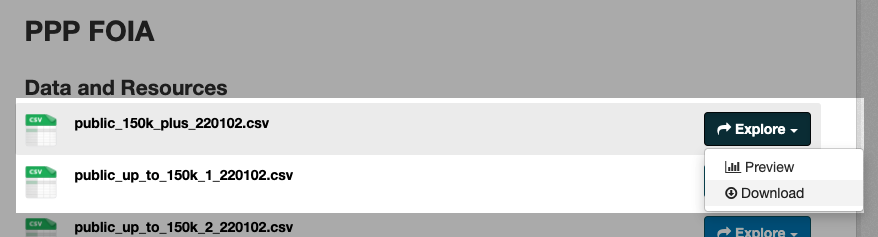
You’ll also want to download the PPP data dictionary at the bottom of the list.
Save the files to your working directory.
Load in the PPP loan data with a function from our Tidyverse package. Again, you can execute the code by clicking “Run” or with CMD + Enter.
#load in our ppp data
ppp_150k <- read_csv('public_150k_plus_220102.csv')
This stores the data in a brand new dataframe named ppp_150k.
We’ll do the same with our data dictionary.
#load in our data dictrionary
ppp_data_dict <- read_xlsx('ppp-data-dictionary.xlsx')
Take note that in your “Environment” window (by default in the top right), you should be able to see your PPP dataframe with 968,538 rows (or observerations) and 53 columns (or variables) and the data dictionary with 53 rows and 2 variables.
Basic gut checks
Before we start working with our data in earnest, let’s get to know it a little bit. You can click on the dataset in your environment window to view it in a new tab in your “Source” pane, much like you would in Excel or some other spreadsheet software.
We can see a number of columns that are pretty self explanatory. Some less so. We’ll need to explore those as we go. Navigate back to your script window, and let’s do a few things to make sure our head is on straight.
For this section, we’ll be using the “pipe” – which looks like this: %>% – to chain together operations.
First, let’s check to make sure we got it all the data when we loaded it.
#how many rows do we have?
ppp_150k %>%
  nrow()
How many states’ worth of data are we looking at? For that, we’ll use the count() function, which accepts one or more fields from our dataframe and… well… counts them.
If we want to know more about a function – for example, the syntax or what sorts of options is has – we can prepend a question mark to trigger the “Help” tab.
#what's up with the count function?
?count()
Let’s check the count with more than one variable.
#are we only looking at NC?
ppp_150k %>%
  count(BorrowerState)

ppp_150k %>%
  count(ProjectState)
Check how much money we’re talking about here? We can find out using the summarize() function, which runs some math across a specified column in your dataframe. Think descriptive statistics: you can find out the sum, max or median across all values, for example.
Let’s start by examining our the InitialApprovalAmount field, which we can see from our data dictionary is definined as “Loan Approval Amount(at origination)”.
#what's our total loan value?
ppp_150k %>%
  summarize(total = sum(InitialApprovalAmount))
Now let’s see how much are borrowers getting on average…
#what about the average?
ppp_150k %>%
  summarize(avg = mean(InitialApprovalAmount))
…vs. the typical/middle value.
#what's the median?
ppp_150k %>%
  summarize(total = median(InitialApprovalAmount))
We’re going to be working with some large numbers here, so let’s disable scientific notation so we can read the output a little better.
#disable scientific notation
options(scipen=999)
Now let’s look at who got the largest and smallest loans using the arrange() function, where we’ll specify we want to see those loan amounts in descending order using the desc() function.
We can also simplify our output a bit to make it a little more readable with a function from the knitr package called kable() which basically just makes are table prettier.
#who got the largest loan?
ppp_150k %>%
  arrange(desc(InitialApprovalAmount)) %>%
  select(BorrowerName, BorrowerCity, InitialApprovalAmount) %>%
  head() %>%
  kable('simple')
%>% symbol at the end of a highlighted section of code. Remember it chains your command to the next line, so RStudio will wait, thinking you're going to enter more code!What about who got the smallest loan amount. That might be a little weird!
#who got the smallest loan?
ppp_150k %>%
  arrange(InitialApprovalAmount) %>%
  select(BorrowerName, BorrowerCity, InitialApprovalAmount) %>%
  head() %>%
  kable('simple')
Although we can see them in the big table view, it might be helpful to get a list of all of our fields in one place so we can see what’s there – and what we might need to ask about during our reporting.
#give me a rundown of the column names
ppp_150k %>%
  names()
Cleaning and grouping
Now that we have a good idea of what’s here, let’s see if we can answer some basic questions about the geographic distribution of these loans. Let’s start with the county (N.C. only), which looks pretty clean.
#group by county
ppp_150k %>%
  filter(ProjectState == 'NC') %>%
  count(ProjectCountyName, name = 'loan_count') %>%
  arrange(desc(loan_count)) %>%
  kable('simple')
But the city is a little different. Notice how often names are misspelled and inconsistent.
#group by city
ppp_150k %>%
  filter(ProjectState == 'NC') %>%
  count(ProjectCity, name = 'loan_count') %>%
  arrange(desc(loan_count)) %>%
  kable('simple')
One thing we can do to fix that is to create a “clean” column, where we use a little code to fix our wonky data. For that, we can use the mutate() function.
Until now, we’ve just been generating output to our comamnds in the Console pane. But we want to make our changes more permanent, so let’s assign that output to a new dataframe.
#create a new dataframe with an attempt to clean up our city name
ppp_150k_clean <- ppp_150k %>%
  mutate(ProjectCity_clean = toupper(ProjectCity)) %>%
  mutate(ProjectCity_clean = str_remove_all(ProjectCity_clean, '\\.')) %>%
  relocate(ProjectCity_clean, .after = ProjectCity)
There are other ways to clean data that we’ll get to in future lessons. But for now, we might make a decision that this is a bit too dirty to work with for the time being.
Joining other data
Among the fields in our data is a column called NAICSCode, which is the code assigned by the North American Industry Classification System. It basically describes what type of business the company is in. The codes are standardized, meaning we can use them to find out how funds are distributed across industry types, but we’ll need to join them up to do that.
First, download our NAICS lookup table here. Then unzip the file and move it to your working directory.
# load in our naics lookup table
naics <- read_csv('naics_lookup.csv')
The dataset we’ll be joining is a lookup table using the first two digits of the NAICS code, which describes the top-level industry type.
First, let’s make sure we have a column to match on.
We’ll use the mutate() function like we did before, but we’ll use it in combination with two other functions: substr() and strtoi(). The first take a “substring” of each NAICS code (just the first to characters of the text). The second converts that text number (a “string”) into an actual numeric type, or an “integer” (strtoi = string to int).
#create a two-digit naics code using the first two positions in our longer naics code
ppp_150k_clean_naics <- ppp_150k_clean %>%
  mutate(NAICS_initial = strtoi(substr(NAICSCode, start = 1, stop = 2)))
There are lots of types of joins, but for this analysis, we’ll use a LEFT JOIN.
Our PPP data is our left table (Table A in the example below), and our NAICS lookup table is our right table (Table B in the example below).
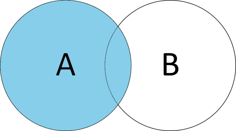
Executing a left join using our two-digit naics code means that only columns from our NAICS lookup table that matches will be tacked on to our PPP data.
The left_join() function accepts a dataframe (naics, in this case) and a by parameter, which tells the function what we actually want to match on.
In this case, the column names we want to match are different. That’s OK! We just use the left table’s column name on the left of the equal sign, and the right table’s column name on the right of the equal sign.
#practice doing a left join
ppp_150k_clean_naics %>% #our leftside table
  left_join(naics, #our rightside table
            by = c('NAICS_initial' = 'naics_initial_code') #our left and right match columns
            )
That output, if it runs correctly, isn’t terribly interesting.
NAICS_initial variable to numeric.There are so many columns, in fact, we can’t even see if the ones we’re interested in (naics_title) are even in the dataframe we created!
So once we know our join works, lets add a little more code to group those results and summarize them into something interesting.
We’ll do that with the group_by() function, which accepts a field/column name and works in concert with the summarize() function to run those descriptive statistics across the group rather than the whole column.
Then we can arrange the result to see the top loan recipients by industry.
ppp_150k_clean_naics %>% #our leftside table
  left_join(naics, #our rightside table
            by = c('NAICS_initial' = 'naics_initial_code') #our left and right match columns
  ) %>%
  group_by(naics_title) %>% #group by our newly joined naics description
  summarize(total = sum(InitialApprovalAmount)) %>% #give us the sum for each group.
  arrange(desc(total)) #arrange in descening order by total
If we want to get really fancy, we can use a nifty function from the janitor package to calculate totals and percentages, then pipe everything to our kable() function to make it extra pretty.
ppp_150k_clean_naics %>% #our leftside table
  left_join(naics, #our rightside table
            by = c('NAICS_initial' = 'naics_initial_code') #our left and right match columns
  ) %>%
  group_by(naics_title) %>% #group by our newly joined naics description
  summarize(total = sum(InitialApprovalAmount)) %>% #give us the sum for each group.
  arrange(desc(total)) #arrange in descening order by total
  adorn_totals() %>% #add a total row at the end
  adorn_percentages('col') %>% #the next three lines format percentages
  adorn_pct_formatting() %>%
  adorn_ns(position = "front") %>%
  kable('simple') #pipe it all into a prettier format
Wrapping up
And there we go!
With a few lines of code, we can quickly see that, at least nationally, the construction industry claimed almost 14% of the initial large loans (those greater than $150,000) through the Paycheck Protection Program, followed by the healthcare and manufacturing industries.
That may be different for North Carolina, or for a specific county and city.
There are certainly more questions we could ask and answer of the data using just these new tools in our arsenal.